I've Got (Graphs for) the Power (Law)

In our last post, which introduced the Power Law, things were getting kinda hectic:




We'd looked at a whole bunch of stats, talked about our friend from high school algebra (formula for slope), and started to repurpose the original gradebook I posted. It was like old home week around here. But we're not stopping there. Nope. It's time to develop graphs for this data. So, let's take a look at the reporting tool in the workbook. I've made a couple of changes.

First of all, because the Power Law focuses attention on the most recent score, the way we look at student progress is going to look different. In fact, if you click on the "Scores" part of the workbook, you'll notice that the columns that used to contain the median scores for a grading period have been removed. In the reporting tool, I've added two items and altered a heading to accommodate the changes. I selected the colour blue to represent "student progress," which is a way to describe the scores determined by applying the Power Law. In other words, black shows the assigned score, and blue the adjusted score. I also replaced the bar chart showing process with the trendline representing the Power Law data. Finally, I changed the head of E10 to be "Learning Trend" instead of "Growth from 1st Quarter."

I'm not going to go through how to create the data validation list for the last name or the whole graph build. If you need a refresher on those items, please (re)visit the Beginner's series Part IIa (data validation, INDEX/MATCH) and Part IIb (graphs). I'm just going to show you the new stuff.

Here's the first row (Row 11) for Steve Canyon's performance. In cell C11, I've used the INDEX/MATCH function to report the most recent score (not an average or median) from the report for this standard. Our "All Scores" graph looks the same as in the original Beginner's Gradebook, but in cell E11, we can see the results of the Power Law plotted out for comparison with a Steve's scores. As you can see, this gives us a different view of student performance. His actual scores jump around, but the overall trend is one of moving toward the standard.

Here are a few other examples for your consideration. In these cases, I've plotted both the student's actual scores (in black) and the predicted scores using the Power Law (in blue).

Gonna Fly Now...

Got Viagra?

Patient flatlining. Clear!

The Power Law can provide a different sort of summary of performance vs. simple measures of central tendency, and can generate different kinds of discussions with stakeholders. Also notice that the learning curve doesn't always head in a positive direction. In the middle example, there's a student who has met standard, but never improved on the performance. And in the bottom graph, you can see that inconsistent performance leads to no curve at all.

Some commercial gradebooks have a Power Law option. It's certainly a lot simpler to have a built-in formula at your fingertips. However, I don't want you to think that you have to spend a lot of money to get this sort of information. And, I firmly believe that you should be in control of your data. You're the expert about your students. You can download the final version of the Power Law Gradebook, which has all of the report completed to use as a model for your own data sets.

Happy dancing!




Music clips from The Power by Snap! (c)1990.

I've Got the Power (Law)

I had a request for an Excel Gradebook that used Marzano's Power Law to determine grades. So without further ado (press play for a musical accompaniment for your continued reading):



You've got the power!

What's the Power Law?
I'm glad you asked, although I don't know a whole bunch about it. If you want a deeper look, check out Transforming Classroom Grading, which goes into the research behind the Power Law of Learning and provides a step-by-step for using it in calculations. But, lemme sum up.

If you were to plot out the scores of a student learning a skill which was brand new to them, which graph do you think would represent their scores over time---the one on the left...or the one on the right?

Inquiring optometrists want to know: "Which looks more clear: #1 or #2?"

Both lines have the same start and end point. They describe the same number of assignments. But one is a better representation for what happens during the learning process. Did you guess the one on the right? Yup. You were correct. When new skills are introduced, there is a big gain in learning at the beginning. With repeated opportunities, learning still increases, but at a much slower rate. Devotees of the Power Law believe that the most recent score for a student is the what should be reported as a grade.

Okay. So now what?
Oh, that student scores followed the exact same trajectory every time. But that's not what happens. Learning is impacted by all sorts of factors both inside and outside of the classroom. The graph above shows the average increase. We need to be able to make an individual student's scores apply to that learning curve. This is where the Power Law comes in handy. Here it is:

Hello...Newman...

It might have been many moons since high school algebra, but perhaps the Power Law reminds you of the one used for slope: y = mx + b. Makes sense as we are trying to look for a trend in learning. In our Power Law formula, y is the student score that is predicted and x is the original student score. The roles of m and b are to act as constants. They take into account the number of scores for a given standard and the position of a score within that range.

Calculating m and b requires some statistics, because in a way, we're "normalizing" the data set to the curve. If it's been awhile since you had to deal with this sort of thing, remember that the "E" symbol means "sum of" and "N" = "Number" (in this case, referring to the number of assignments for a given standard. Don't get too sweaty looking at these, because our buddy Excel is going to do all of the heavy lifting for you. I just want you to see them before we look at the gradebook.

omgwtfbbq

And now, a musical interlude:



Back to our regularly scheduled workbook...

I'm going to build this workbook using the finalized Excel for Beginners workbook. Keep in mind that these formulas will work the Intermediate and Advanced versions, too. Just plop the formulas any old place and they'll do your bidding. Here is the first chunk of student scores:

Now, we need to transform them using the Power Law. I've set up a column for the variables we're going to use: x = (natural log of) Assignment #, y = (natural log of) Student Score, then the various combos we'll need using these. Please note that the y here is not the same as the one in the Power Law itself---it is just a statistical variable assigned to calculate m and b. (Confused yet?)

And here are the formulas generating these values:

I've probably made this look far more complicated than it needs to be, but I also like the idea of breaking down the steps---especially if you're new to Excel or just need the opportunity to follow along with what is happening. The formulas in D26 and D27 use the natural log (LN) to transform the ordinal number of the assessment (x) and the student score on that assessment (y). Cells D28 - D34 are used to process x and y so they are ready to use in our equations for m (D35) and b (D36). The "predicted score" showing in Row 22 shows you the result of the Power Law formula (y = mx^b) for each student score.

Here is the link for the Power Law workbook with formulas. We'll talk about the graphs for this function in the next post, as well as reveal the final version of the workbook. Download this one first so you have something to play with.

Now, come on and sing it with me:



Bonus Round
Want more of The Power by Snap! to listen to while you work on your gradebook? Cue this up.

Share Your Wealth of Data Knowledge

Do you have mad skillz when it comes to Excel, SPSS, or other data tools? Know a regression from a box plot? Are you anal retentive when it comes to cleaning and organizing data sets?

Then you should consider becoming a volunteer for Data Without Borders. From their site:

Data Without Borders seeks to match non-profits in need of data analysis with freelance and pro bono data scientists who can work to help them with data collection, analysis, visualization, or decision support. Big companies like Google and Amazon recognize the importance of dedicated data science teams and can support fulltime analysts, but non-profits, though they may have rich and interesting datasets, don’t have the resources to capitalize on their data or may not even know the value of the data they already collect. Data Without Borders aims to close that gap through a data scientist exchange, bringing exciting new problems to the data community and helping to solve social, environmental, and community problems alongside nonprofits and NGOs.

They have a Datadive coming up in San Francisco early in November. I watched the NYC Datadive recently, and was both fascinated and deeply heartened by the work that weekend. You can check out the project wiki here. It provides you with links to each of the presentations by the NGOs/non-profits, as well as project pages where you can get an idea of the scope of the work that was completed 48 hours later.

Data Without Borders has many different options for volunteers. So, if you're not into coding, don't know a bar graph from a pie chart, or are prone to fainting at the sight of a normal distribution, fear not. There are still opportunities for you to support others in this work.

Report Card Redesign

You might be interested in the Redesign the Report Card contest happening over at Good. You can vote on one of seven entries through Sunday, October 23.

The standard report card is in need of a major redesign. Grant Wiggins once opined that report cards should be more like baseball cards. I agree. Not only has the basic report card format remained more or less unchanged over the last 150 years, it rarely reflects the whole child. While the Roll Your Own Gradebook series here is an attempt to look at a different way to display student data, it is only a first step toward giving teachers control of the data they have and how they share meaning with others. We still have a ways to go to making things pretty.

But click on over and take a look at what has been suggested. Here are the two I liked best.

This submission, by Polly Avignon, uses colour-coding for assignment categories and simple graphics to communicate a variety of data: scores, attendance, observations. (Click here for a larger version.)

I also like this one by Larry Buchanan (larger version here):

Although I personally wouldn't choose to display the class average (or any average at all, for that matter), I do like the area graph with comments. I also like the separation of grades from student behaviors, such as participation and effort.

What do you see that you like?

Excel Gradebook for Advanced Users: Nested IF Statements

And now, the grand denouement of the Roll Your Own Gradebook series. If you're new around these parts, you can catch up on the series with

• Beginners, Part I: Organizing Data
• Beginners, Part IIa: INDEX and MATCH
• Beginners, Part IIb: Sparklines
• Intermediate, Part I: Ranges and Validation Lists
• Intermediate, Part II: Using the IF Function
• Intermediate, Part III: Building Dynamic Graphs

Each comes with a screencast tutorial and links to both the "before" and "after" version of the gradebooks. Make classroom data dance to your tune and shake its little moneymaker for your stakeholders using Excel.

In the intermediate series, we integrated two sets of data into one report. But let's face it, most teachers do not have the luxury of teaching two classes or subjects. If you're an elementary teacher, you're juggling multiple subject areas and assessment sources. Secondary teachers have several class periods. You can still use a single reporting tool. You just have to master one more formula: the nested IF statement.

You already know how to construct an IF statement. In fact, if you've been following this series, you've already done a fairly complicated one involving the addition of INDEX and MATCH. This time, we're just going to expand that to "nest" (read: embed) a couple more IF statements in the formula. You can download the gradebook for this tutorial here.

In this workbook, there are 4(!) classes. We still have biology and chemistry from the intermediate series, and now we have physics and earth science. We also have the same Report we've been using since the very beginning. I've already added the named ranges for you in the Formulas worksheet. You will not need to update the data validation lists for the report.

In the Intermediate gradebook series we used the following formula to fill in the cell marked in yellow: =IF($C$4="P1 Biology",Formulas!B2,Formulas!C2)

We had two classes, which fit perfectly into the plain Jane IF statement: a place to tell Excel to look if the first part ($C$4="P1 Biology") was true (the first cell with a biology standard), and a place to look if the first part was false (the first cell with a chemistry standard).

Now, we have to tell Excel to look in one of four places. Oh noes! It doesn't fit in an IF statement anymore. But we can fool Excel with an Inception-style solution: an IF statement within an IF statement within an IF statement.

Here's what it will look like: =IF($C$4="P1 Biology",Formulas!B2,IF($C$4="P2 Chemistry",Formulas!C2,IF($C$4="P3 Physics",Formulas!D2,Formulas!E2)))

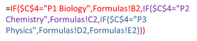
Here's what it means. The red text below shows the beginning of our IF: the statement to evaluate ($C$4="P1 Biology") and what to do if that is true (Formulas!B2), but instead of directing Excel to another cell for a false statement, we feed it another IF. This is the statement in purple, which leads to another false statement in blue. Once you have this formula in place for the report, use your fill down option (look for the crosshairs when your cursor is placed in the bottom righthand corner of the cell) to complete the three cells below.

That's not so bad, is it? Keep in mind that you can have up to 7 IFs nested in a single statement. If you have more than 7 options, you will have to use a workaround that we can talk about in another post.

Okay, now you need to take a deep breath and modify the IF/INDEX/MATCH statement from the Intermediate series of tutorials. The bad news is that this is going to look a little scary. The good news is that you only have to do it once. After that, you can copy and paste the formula into other cells, then just edit the columns you need.

Let's start with the box for the student's first name, shown in yellow in the diagram shown below.

In the Intermediate series, we used the following formula: =IF(C4="P1 Biology",INDEX('P1 Biology'!B8:B17,MATCH(C6,P1Biology,0)),INDEX('P2 Chemistry'!B8:B17,MATCH(C6,P2Chemistry,0))). This time, due to juggling four classes, you're going to have to manage a much larger formula. You've trained for this. You can do it.

Ready? Okay!

=IF(C4="P1 Biology",INDEX('P1 Biology'!B8:B17,MATCH(C6,P1Biology,0)),IF(C4="P2 Chemistry",INDEX('P2 Chemistry'!B8:B17,MATCH(C6,P2Chemistry,0)),IF(C4="P3 Physics",INDEX('P3 Physics'!B8:B17,MATCH(C6,P3Physics,0)),INDEX('P4 Earth Science'!B8:B17,MATCH(C6,P4EarthScience,0)))))

It's not as bad as it looks. See the pattern? IF, INDEX, MATCH...IF, INDEX, MATCH...Lather, Rinse Repeat. And you know what? For all the "Current Scores" cells, you only need to change the highlighted columns in the formula.

When you're ready to fill in the formulas for the dynamic graphs, you can copy and paste the formula again, but you will have to make a couple of adjustments. Excel won't know that cells C4 and C6 refer to the Report worksheet unless you tell it. To make the fill go more easily, make some attributes absolute (with the $) so that Excel only changes the columns you want it to change. Here is an example for cell H2 of the Formulas sheet:







=IF(Report!$C$4="P1 Biology",INDEX('P1 Biology'!C$8:C$17,MATCH(Report!$C$6,P1Biology,0)),IF(Report!$C$4="P2 Chemistry",INDEX('P2 Chemistry'!C$8:C$17,MATCH(Report!$C$6,P2Chemistry,0)),IF(Report!$C$4="P3 Physics",INDEX('P3 Physics'!C$8:C$17,MATCH(Report!$C$6,P3Physics,0)),INDEX('P4 Earth Science'!C$8:$C$17,MATCH(Report!$C$6,P4EarthScience,0)))))

Also remember that not every class has the same number of scores to report for every standard. For example, cell O2 of the Formulas sheet would use

=IF(Report!$C$4="P2 Chemistry",INDEX('P2 Chemistry'!J$8:J$17,MATCH(Report!$C$6,P2Chemistry,0)),IF(Report!$C$4="P3 Physics",INDEX('P3 Physics'!J$8:J$17,MATCH(Report!$C$6,P3Physics,0)),""))

because only the Chemistry and Physics worksheets have assignment scores in Column J (Biology and Earth Science have median scores in those columns). The "" at the end of the formula tells Excel to leave the cell blank if it is not a Chemistry or Physics class. If you're still a little confused about this part, you might want to go back and review the last part of the Intermediate series.

Want to check your work or just don't want to hassle with building the workbook? You can download a copy of the completed version of this gradebook (with all of the formulas and graphs).

Here is the YouTube version of the tutorial. Enjoy!



Don't be sad that we have reached the end of the gradebook build. There will be plenty of new permutations to explore. (I've already had an inquiry about adding in the Power Law formula.) We will also look at other types of dashboard reports to summarize activity in your classroom. Keep leaving your ideas and suggestions in the comments and we'll keep on trucking with this.

Bonus Round
Does the thought of managing these formulas make you queasy? Remember that you can just use what's included with the Beginner's series and create a separate workbook for every class or subject. Or, if you have more than one period of the same subject, list all students in the same worksheet. This will decrease the number of IF statements you need to develop.

How Stacked Bars Stack Up

I'm starting to put together a workshop on Excel dashboards that will be in December. I'm playing around with a few different data sets and options, and have a quandary I'd like your help with: What is the best layout option when using stacked bar charts?

If you don't know what a stacked bar chart is, here is an example:

There is one bar representing 100% of whatever is being measured: numbers of students, percentage of scores, speeds of African and European swallows, and so forth. In the stacked bar chart shown above, there are four categories which have been numbered. Instead of each category having its own private bar, they get together and party in one space. The size of the categories, indicated by different shades of green in the example, shows their proportion of the 100%. It is a simple way to compare the relative sizes of categories...and all without some ridiculous pie chart.

But stacked bar graphs do not have to take things lying down. They can be vertical, too. Which leads me to my problem: When should you use the horizontal format...and when should you use the vertical format? My Google Fu hasn't turned up any rules. Seems like everyone is just letting it all hang out.

There are three layout options shown below. I know I don't have the categories labeled, but I just want to consider layout at the moment. Just FYI, the data represent scores on the 2011 Washington state test for reading. The shades of green, from lightest to darkest, show the percent of students at a school who scored at Levels 1, 2, 3, and 4.

The first layout has a very traditional look:

Labels for each grade are to the left. The graphs are (more or less) placed so that you can make a quick comparison among the grade levels. But is this better?

Same data. Same graphs. Just rotated 90 degrees. I don't know about you, but I find this easier to "read" when looking across the grade levels. It's true that there would be some issues with how closely the graphs can be pushed together due to the labels, but the overall format is okay.

And finally, my least favourite, but deserving of discussion is this:

 

Considering that there will be more graphs for mathematics, science, and writing, would it be more important to look at performance for a subject area across and review data for a grade level along a vertical axis (not shown here, but imagine there are stacked bar charts for the other subject areas underneath). 

What do you think? Just from the standpoint of layout, which format is most meaningful for you?

The Most Wonderful Time of the Year

Welcome to Spreadsheet Day 2011 on Excel for Educators. Personally, I think every day should be Spreadsheet Day. But then, I was also disappointed when I couldn't change my Facebook status to show that I am in a relationship with Excel.

The theme of this year's Spreadsheet Day is to help students. I have been traveling for work the past two weeks, and so my preparations for this day have not been made. I will, however, have a post later this week which finishes fleshing out the standards-based gradebook for teachers.

What I would like to share today, however, is a word of encouragement. You see, Excel and I were not always BFFs. In fact, I used to be afraid of even clicking on its weird-looking green alien icon. And then I found myself teaching a class where we were going to help chemistry students do a regression. I had to man up, as it were, and dive into the world of spreadsheets. And I've happily been there ever since.

I wish I had known all of the things I could have done with Excel to help me as a teacher. Not only for tracking student scores, but for all types of record-keeping: attendance, calls to parents, student behavior notes, observations, tracking time for lessons. I could have used the graphs to look more closely at student grades and reflect on what was happening. And, I could have helped students do more with Excel. I was a science teacher, for crying out loud. We could have integrated spreadsheets with so many labs.

So, my advice for today is simply to go forth and double-click. Open Excel and play around. Think about the ways it could automate some of the tasks for your classroom and change your workflow. And if you don't know how to make Excel bend to your will, ask me or someone else who can help. We'll learn with you. Can you think of any better way to model the power of spreadsheets for your students?

Update: Visit the Contextures Blog for the full round-up of Spreadsheet Day posts.