Statistically Speaking with Excel: Basic Descriptive Stats

If you want to do some heavy statistical analysis, there are better programs than Excel for doing so. But, let's say that you aren't into #bigdata and just want to do some small scale divination. Excel can totally be your bff for that.

Educators are most familiar with descriptive statistics: the ways we describe a set of data. What is the shape of the distribution of values? Where is the "middle"? What can we say about the population of values and their relationship to one another?

I have pulled a new data set to play with...one with test scores for about 500 students. While you can do statistical analysis with your gradebook---and let's face it, most teachers do in terms of how they assign final grades for students---I am a little squeamish about doing so. There may be no magic number that applies to every sample size, but I want us to play with something we can have a little more confidence in than the basic gradebook I've posted here. You can download the test scores workbook here.

This is the basic set up:

I have divided the data set into two schools: A and B. Each student is identified by their first name, and in some cases, a last initial. There is a raw score for reading, writing, and math, as well as a level of performance (1, 2, 3, 4). The range of score points for each level plays out like this:

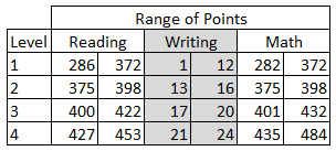
You may look at this and wonder about what appears to be missing points (Why can't anyone get a 399 on the reading or math test?!) and why writing has a different scale. There are reasons...good ones...but I'm not going to get into them at the moment. These data do come from (old) state test results: first names of students are unchanged, but I did fill in some missing scores. We're going to play along with the rules that were originally applied to determine the scores. So, do your best to overlook the oddities of these scales for now. For these tests, a score in Level 3 would mean a student can meet the standard (Level 4 = exceeds, Levels 1 and 2 = below standard).

Let's start with measures of central tendency (mean, median, and mode) for our reading data (C2: C517). For the mean, Excel uses the AVERAGE function...for median, oddly enough, we can use MEDIAN...and for the mode, it depends on which version of Excel you have. In olden versions, the MODE function worked just fine, but starting with 2010, you have choices. To just get "the" mode, use the MODE.SINGL function. To get multiple modes from an array of data, you can use the MODE.MULT function---a very handy improvement. Not every data set is bell-shaped. So, here is what we have for the reading scores. I placed the formulas in the table on the right so you can see the syntax.

What does this mean? Well, first of all, our mean, median, and mode are all about the same. It's not necessary for your measures of central tendency to agree. After all, each one is a different way to identify the "middle." It's up to you to determine which is most appropriate. However, in this example, no matter which one you choose, you'll be fine.

If you want to graph this data set, it's not so friendly in its current form. We'd be better off building a frequency table first. This will allow us to find out how many students are in each category, then create a graph to visualize the distribution. To keep things simple, let's find out how many students scored in each level for the reading test. Build a simple table first, then select the empty cells:

Now you're ready to add your formula---a single formula ("array formula") which will fill all the cells at once. Then belly on up to the formula bar (too bad you can't pull a beer from here) and start entering the formula:

The "data_array" will be the column of data (not including the header) with the data about reading levels. The "bins_array" refers to the cells that have the labels for the reading levels---in this example, the 1, 2, 3, 4 you see in to the left of the cells selected in the table above. The final formula looks like this (plus a close parenthesis at the end):

When you've finished entering this information, you need to use a command to fill in all of the cells in the table. Plain old ENTER will not work. You have to use CONTROL + SHIFT + ENTER. And poof! We now have a frequency table:

If this scares you, you can use a simple COUNT function in each cell, but hey, you're ready to use big kid functions. Give FREQUENCY a try. Use the filters in Excel and compare School A with School B.

This is a good spot to stop for today, but we'll come back to this data set another day to see other descriptive statistics in Excel...and then move on to inferential analysis.

Bonus Round
Did you know that Excel has a whole category of statistics functions? Get in there and play!

Adding IFERROR to Your Excel Diet

There are a lot of Excel tips and tricks out there---whole blogs, YouTube Channels, message boards, and more devoted to all of the things that make Excel such a versatile piece of software. While the purpose of this blog is not to replicate all of that amazing content, I do want to pull out ideas and functions that educators might find the most useful.

Have you ever set up an equation in Excel and gotten an error message---such as #N/A, #VALUE!, #REF!, #DIV/0!, #NUM!, #NAME?, or #NULL!? Total buzzkill. On one hand, these alerts serve a greater good. They let you know if your formula has gone awry. And, on the other hand, they can show up in an embarrassing places.

In our Roll Your Own Gradebook series, we made the assumption that we had classes of Stepford children: every student completed every assignment. But let's face it, that's not what really happens. For example, let's say that Flash Gordon wasn't enrolled in the course for the first quarter. If there are no scores, then Excel gives us an error message when it tries to apply the formula:

Uh-Oh, Spaghetti-O

You can change this, without altering the outcome for other students, by using IFERROR. This function tells Excel to evaluate what's happening, placing one value in the cell if there's no error (e.g. score for Stepford child) and another if there is an error message (e.g. "Trash" Gordon, lazy athlete). In short, it allows you to bypass the error message.


How It Works
You could apply the formula to more than one location in the gradebook and get the same result, but for now, let's look at the worksheet with the scores.

Superhero Behaving Badly

The cell on the right---the one with the "###" is the one we need to address. The current formula is =MEDIAN(H14,J14). Alas, there are no scores to find the median for---hence the error.

Instead, we can use =IFERROR((MEDIAN(H14,J14)),"") The double double-quotes at the end tell Excel to leave the cell blank. However, you can put another value there or even a text string (e.g. "No Grade"). Here is what we see now:

Ahhh...That's Better

What do we see on the Dashboard?

A blank. Wow. Excel is doing just what we told it to do. Imagine that.

Excel Gradebook for Beginners, Lesson One: Organizing Data

This is the first in a series of posts (also available over at What It's Like on the Inside) on building your own gradebook. If you're not into the whole gradebook idea, I'd encourage you to keep reading, anyway. The tips and formulas would be just as useful for whatever data set(s) you are managing. Are you an elementary teacher who DIBELs? In a school with MAP testing? A district with various benchmark or interim assessments where you want to look at performance by classroom or school? If you've got a list of students/teachers/schools that has data next to it, then, these ideas are for you, too.

One of the most frustrating things (for me) as I try to do new things with Excel is the lack of non-business examples. Most websites and YouTube videos assume that you are (a) always working with numerical data and (b) interested in some sort of angle about profit margin or losses. We really do need a bank of "how to's" that models for education. If you have seen some, please do share in the comments.

I've had a lot of you contact me over the summer asking about my Excel gradebook and any updates. I have been promising to post those...and now your wait is over. The video below will show you how to get set up. I also have a sample workbook you can download and use with the video. (But if you want to use your own data sources, that's cool, too.)

As you will see, the workbook has two worksheets: Scores and Report. This allows me to keep the raw data separate from the dashboard reporting too. Depending upon what you're working with, additional sheets can come in very handy. Perhaps you want them for qualitative data you collect, attendance, discipline, or other notes. If not, and you're anal-retentive about how your spreadsheet looks, then an extra sheet is very handy for stashing your formulas and ranges: It will keep your raw data looking fresh and clean. If you're hellbent on making things look pretty, stay tuned for later videos. You'll have the Miss America of dashboards when I'm done.

I populated the Scores worksheet with some names, assignments, and data. Even though the default color themes in Excel are awful, I demo them so you can see some basics about applying colour. I like to separate grading periods and different types of standards using colour. This makes it much quicker to find information. But I also apply conditional formatting to the spreadsheet so that I can more easily visualize what is happening with the scores. Finally, I use a simple formula to determine the median and help summarize the scores.



In the next session, I'll show you how to create a dropdown list of student names. The selection from the list will be used to auto-fill many of the cells in the reporting tool using a formula with INDEX and MATCH functions. Sound like it's over your head? Come back and give it a try. I think you'll be surprised at just how easy it is.