The Perfect Match

Heading back into the mailbag, Alison sends us this problem: I have some students with the same last name and the index/match doesn't seem to be doing what I need it to.  It's only finding the first name in the list with that last name.  So I can pull the report for Y. Gordon in 1st period, but not T. Gordon down in 4th period.

I pointed her to Debra Dalgleish's post from July that does a lovely job of showing how to check multiple criteria with INDEX and MATCH, but Alison still felt a bit overwhelmed. I knew what she meant. Sometimes, it's hard to translate an example that doesn't look like yours into the problem you're trying to solve---even when the formulas are the same. So let me share a classroom example.

We need some music to set the stage for our Match Game, don't you think?

Here is our class list. We have a Charlie and Sally Brown in the same class. Ditto for Linus and Lucy Van Pelt. If we want to build a report or find scores, we can't just use the last name to find a student. This isn't unusual for any given class--and while you might end up with a class list of unique last names, you are more likely to end up with 2 or more kids with the same first name.

The easy way out of this problem when building reports is to use the student number or another unique identifier for each student. Then, just use your regular INDEX/MATCH coupling to drive the report. But we're not taking the low road today, my friends.

Suppose we're building a report and need to find the score for each student at the end of the quarter (Column J). For the purposes of this example, we'll use cell C16 on the Report page (Report!C16) as our reference for a cell that already has the last name of a student.

Ordinarily, we might build a formula like this: =INDEX(J8:J17, MATCH(Report!C16,A8:A17,0))

We tell Excel to INDEX the range of scores for second quarter (J8:J17) and MATCH our reference cell (Report!C16) with the list of student last names (A8:A17). Alas, this isn't going to work if we need to find scores for Sally Brown or Lucy Van Pelt. Excel is going to stop when it runs across the first instance of the last name "Brown" or "Van Pelt."

We're going to need an array formula to do some heavy lifting here. Remember, these are formulas where you have to use CTRL+SHFT+ENTER (not just ENTER) to get them to work. This formula is structured very similarly to the plain Jane version.

To keep things simple for this demo, let's say that the formula is going in cell J19 for Sally Brown. (Yes, I know you would just look it up if you were on the same page. Work with me here.) Here is our new and improved INDEX/MATCH formula:

=INDEX(J8:J17,MATCH(1,(A19=A8:A17)*(B19=B8:B17),0))

We're still INDEX'ing the same column (J8:J17), but we're going to shake up the MATCH part of the equation to connect with two variables. We set up one set of matchmaking between cell A19 (Brown) and the range with the last names (A8:A17) and another between cell B19 (Sally) and the range with first names. In between, we put a "*" to direct Excel to combine these values.

Want to play with it? Have it in the embedded worksheet below. Change the names and watch the magic happen.

You can also click the Excel icon at the bottom of the window to download the workbook.



Bonus Round
Have an Excel question you want to air out here?  Drop me a line. I do have a couple more unanswered comments from previous posts to respond to...so if you've been waiting for an answer, stay tuned.

The Back End of the Shaggy Dog

I work in tech, and people are forever referring to the "back end" of software, databases, and so on. I find the reference amusing (because inside, I'm 12), but I have to admit that the euphemism fits. The code, meta-data, and other unseen features are not the pretty face that gets shown around. So let's take a look behind the scenes, as it were, of my Shaggy Dog Story with Excel.These instructions are all about MacGuyvering a spreadsheet. While I hope that no one needs them "as is," there are a few tricks here that you might find handy for other projects.

First, I organized my resources on one spreadsheet. Then, I made it into a table. You can do this in Excel by clicking in the cell that will be the uppermost lefthand corner of the table, then using CTRL+T. My table had headers (unit, resource, title description), so I checked that box and hit ENTER. You don't have to turn the data into a table, but (1) I think it makes the formulas easier to manage and (2) you don't have issues with adding records.

Now I have something that looks like this. If you don't like the formatting Excel applies, you can go into the Table options and fuss around with it.

Then, set up your sheet where you want the results displayed. If you're using Excel offline, just use data validation. Don't bother with my "X marks the spot" strategy. However, if you're trying to webify this content, carry on. This is how I set up the demo for the blog post. I used the four column headers (in brown) on this sheet to organize the display.

There are two more small pieces before we get knee-deep with generating a list of items based on user input. First, on the sheet with the list of resources, I set up two IF statements, one for the choices underneath "Unit" and the other for "Category." I needed to tell Excel how to recognize the selections made by the user. Here is how I set up the formula for Unit:

This formula is placed on the other sheet, but since cell references are on this one, I'm showing it here.

Keep in mind that if you're building an offline version using dropdown menus, you can skip this part.

Finally, I set up a COUNTIFS statement based on the user selections. This was also placed on the page with the data set: COUNTIFS(List[Unit],G2,List[Category],G3). This tells Excel to count all of the cells in the table that matched the results of the two IF statements. I named this formula Item_Count. The one I did for work ended up with nearly 30 choices and two extra layers of IF statements...but we won't bother about that now.

An aside here...

I mentioned earlier in the post that converting the data into a table made things simpler for the formulas. Notice that in the COUNTIFS formula that I don't need to state a particular range (e.g. A1:A50). I can just tell Excel to use the table (List) and column header in square brackets (Unit, Resource).

Okay, let's go back to the sheet with the results. We have one more formula to apply...and it's a doozy. Why? We need to generate a list of results based on user input. Our old friends, INDEX and MATCH, are great at identifying the one item that fits a set of criteria...but we need a list. We need Excel to find the first one, the next one, the next one...and so on. Also, the results of each list might not be the same in number--could be one item, could be ten.  I found the basic answer here, if you want to watch a video tutorial; but here's the basic idea for cell B11 shown below. Keep in mind that this is an Array Formula, which means you need to use CTRL+SHFT+ENTER to make it work.

=IF(ROWS($B$11:B11)>Item_Count,"",INDEX(List[Title],SMALL(IF(List[Unit]&List[Resource]=List!$G$2&List!$G$3,ROW(List[Unit])-ROW(List!$A$2)+1),ROWS($B$11:B11))))

If you're hyperventilating after looking at that formula, find a paper bag and come back. We can do this.

The first part of the formula (=IF(ROWS($B$11:B11)>Item_Count,"") means that we want Excel to count the rows from B11 to B11 and compare them to the result of the COUNTIFS formula (named "Item_Count"). If there are more rows than the Item_Count, Excel should leave the cell blank. This part is important because we are going to have a variable number of results based on user input. By including the option for the blank result, we will keep error messages from showing up.

Next, we have the FALSE part of the IF statement---what Excel should do if the Item_Count is smaller than the number of rows. In this case, I want it to INDEX the Resources and display the title based on the following criteria:

• It must match both the Unit and Category as indicated by the results of the IF statements we set up earlier. (IF(List[Unit]&List[Resource]=List!$G$2&List!$G$3)
• It must be the "smallest" (first) item that matches the criteria that is equal to the number of rows we've specified +1:  SMALL(IF(List[Unit]&List[Resource]=List!$G$2&List!$G$3,ROW(List[Unit])-ROW(List!$A$2)+1),ROWS($B$11:B11))

The good news is that you only have to build this formula once. And trust me, you will do your Happy Dance when it works. Use your fill tool to copy the formula down. You can also copy and paste the formula to cell E11 for the description, then change "List[Title]" to "List[Description]" in the formula.

You can download the workbook here, or go back to The Shaggy Dog Story and see how things work in the embedded version.

See? That isn't so Ruff! Ruff!

Bonus Round
The gigantic formula shown above has a lot of different uses. Don't discount it just because it looks scary. For example, think of how you might use it to sort a list of students into different classes (i.e. take a master list and sort it onto multiple spreadsheets). Although Excel is not a database tool, this formula gives you some options to use it that way when you need to.

Statistically Speaking with Excel: Basic Descriptive Stats

If you want to do some heavy statistical analysis, there are better programs than Excel for doing so. But, let's say that you aren't into #bigdata and just want to do some small scale divination. Excel can totally be your bff for that.

Educators are most familiar with descriptive statistics: the ways we describe a set of data. What is the shape of the distribution of values? Where is the "middle"? What can we say about the population of values and their relationship to one another?

I have pulled a new data set to play with...one with test scores for about 500 students. While you can do statistical analysis with your gradebook---and let's face it, most teachers do in terms of how they assign final grades for students---I am a little squeamish about doing so. There may be no magic number that applies to every sample size, but I want us to play with something we can have a little more confidence in than the basic gradebook I've posted here. You can download the test scores workbook here.

This is the basic set up:

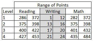
I have divided the data set into two schools: A and B. Each student is identified by their first name, and in some cases, a last initial. There is a raw score for reading, writing, and math, as well as a level of performance (1, 2, 3, 4). The range of score points for each level plays out like this:

You may look at this and wonder about what appears to be missing points (Why can't anyone get a 399 on the reading or math test?!) and why writing has a different scale. There are reasons...good ones...but I'm not going to get into them at the moment. These data do come from (old) state test results: first names of students are unchanged, but I did fill in some missing scores. We're going to play along with the rules that were originally applied to determine the scores. So, do your best to overlook the oddities of these scales for now. For these tests, a score in Level 3 would mean a student can meet the standard (Level 4 = exceeds, Levels 1 and 2 = below standard).

Let's start with measures of central tendency (mean, median, and mode) for our reading data (C2: C517). For the mean, Excel uses the AVERAGE function...for median, oddly enough, we can use MEDIAN...and for the mode, it depends on which version of Excel you have. In olden versions, the MODE function worked just fine, but starting with 2010, you have choices. To just get "the" mode, use the MODE.SINGL function. To get multiple modes from an array of data, you can use the MODE.MULT function---a very handy improvement. Not every data set is bell-shaped. So, here is what we have for the reading scores. I placed the formulas in the table on the right so you can see the syntax.

What does this mean? Well, first of all, our mean, median, and mode are all about the same. It's not necessary for your measures of central tendency to agree. After all, each one is a different way to identify the "middle." It's up to you to determine which is most appropriate. However, in this example, no matter which one you choose, you'll be fine.

If you want to graph this data set, it's not so friendly in its current form. We'd be better off building a frequency table first. This will allow us to find out how many students are in each category, then create a graph to visualize the distribution. To keep things simple, let's find out how many students scored in each level for the reading test. Build a simple table first, then select the empty cells:

Now you're ready to add your formula---a single formula ("array formula") which will fill all the cells at once. Then belly on up to the formula bar (too bad you can't pull a beer from here) and start entering the formula:

The "data_array" will be the column of data (not including the header) with the data about reading levels. The "bins_array" refers to the cells that have the labels for the reading levels---in this example, the 1, 2, 3, 4 you see in to the left of the cells selected in the table above. The final formula looks like this (plus a close parenthesis at the end):

When you've finished entering this information, you need to use a command to fill in all of the cells in the table. Plain old ENTER will not work. You have to use CONTROL + SHIFT + ENTER. And poof! We now have a frequency table:

If this scares you, you can use a simple COUNT function in each cell, but hey, you're ready to use big kid functions. Give FREQUENCY a try. Use the filters in Excel and compare School A with School B.

This is a good spot to stop for today, but we'll come back to this data set another day to see other descriptive statistics in Excel...and then move on to inferential analysis.

Bonus Round
Did you know that Excel has a whole category of statistics functions? Get in there and play!